8.6 Head loss

Head loss in straight pipes

Head loss is energy loss due to friction in pipes, fittings, valves, heat exchangers and other components connected to the piping system. The energy lost was originally added to the fluid by the pump, hydraulic energy. There are basically two methods used to calculate head loss in fully charged circular pipes.

The Hazen Williams method is valid for head loss calculation of water in a cast iron pipe. There are correction factors available for other pipe material as well but since it is limited to water it is mostly used in water distribution or fire sprinklers.

The Darcy Weisbach method can be used for any Newtonian fluid in any pipe material and for turbulent or laminar flow. The method has no limitations for incompressible fluids but if used for compressible media like gases or vapors limitations in accuracy applies.

• If pressure drop between system inlet and outlet (P_in – P_out) < 10% then we can expect reasonable accuracy
• For pressure drop 10% < (P_in – P_out) < 40% , use average fluid density at the inlet
• If  (P_in – P_out) > 40%, do not use the Darcy Weisbach method

The following formula applies to head losses for flow in a straight pipe using the Darcy Weisbach method:

h_L = head loss (m)
λ = loss coefficient
l = length of pipe (m)
d = diameter of pipe (m)
v = flow velocity (m/s)

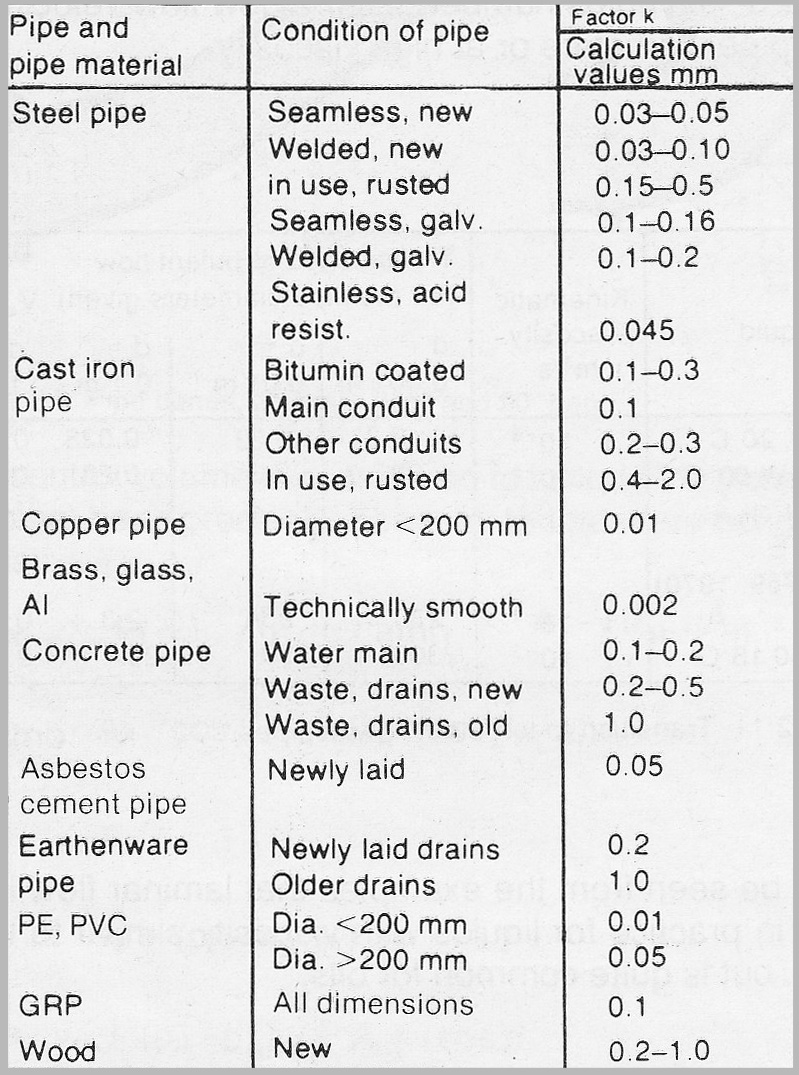
The loss coefficient λ is dependent upon Reynolds (see more about Reynolds number in previous section Pipe flow loss>>> ) number and upon the internal roughness of the pipe. This is shown in the diagram below.

The roughness of the pipe can be asserted from the values in figure 8.6b. The loss coefficient λ can also be calculated from the following formula:

Laminar flow Re < 2300

λ = 64/Re     (Equ. 8.6b)

Turbulent flow Re > 4000

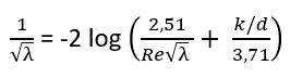
Equation 8.6c is sometimes called the Colebrook-White formula. In the region Re = 2 300 to Re = 4 000 laminar and turbulent flows may alternate in various sections of the pipe. The resultant loss coefficient will then assume values between those obtained in formula 8.6b and 8.6c.

Figure 8.6b Examples of approximate roughness in pipes

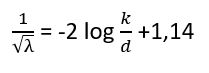
The 8.6c expression is somewhat inconvenient for manual calculation. Within that region in the diagram (figure 8.6a) where λ is independent of Re, the following simpler formula 8.6d can be used:

Other formulae which often occur in literature for the calculation of straight pipe losses in the turbulent region are the so-called Hazen-WiIIiams and Manning formulae. These, however, do not provide any additional information to the equations presented above. They are not dimensionally consequent and have, therefore, been omitted.

Head losses in fittings

Head losses in bends, valves, etc. can be calculated with the help of this formula:

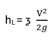
ζ = loss coefficient for fittings, valves etc.
v = flow velocity (m/s)
g = 9,806

The magnitude of the head losses are in principle influenced, as in the case of straight-pipe flow, by surface roughness and by Reynolds number. Examples of approximate values of loss coefficients for losses in fittings are illustrated in figure 8.6c.

All values are those for conditions of normal roughness and at high Reynolds number, i.e. at fully developed turbulent flow.

In cases where the velocity alters it must always be the highest velocity which is used for calculating h_L in accordance with equation 8.6e. In the case of varying diameters, the velocity to applied is the one resulting from the smallest diameter. In the case of T- pipes, the velocity Related to the total volume flow is applicable.

Figure 8.6c Approximate values for loss coefficients for head losses in fittings. The values for loss coefficients in flowmeters are stated in Section 8.10.

An alternative method of expressing the magnitude of head losses in fittings is the use of the concept of equivalent pipe length, l_eq, i.e. the equivalent length, (l_eq) of straight pipe giving rise to the same losses in pressure as the bend, at the same flow velocity. By comparing Equations 8.6a and 8.6e we get:

l_eq = (ζ / λ) * d        (Equ. 8.6f)

lt can be seen from Equation 8.6f that the equivalent pipe length is a function of λ, i.e. the surface roughness of a straight pipe and Reynolds number. It is therefore difficult to quantify l_eq as a specific property for, say, a pipe bend and is thus of an approximate character. For λ = 0.02, the equivalent pipe length of a 90° bend with short radius (r = d) is l_eq = 20 * d.