
3.1.6 Centrifugal pump curves
Centrifugal pump curves
Centrifugal pump curves define the centrifugal pump hydraulic performance and its efficiency. The hydraulic components are head (meters or feet), flow (m³/s or gpm) and NPSH (meters or feet). In addition, pump efficiency (η) as a quote of energy loss in the pump has its own curve. Head is the height of the pumped liquid (pumpage) column that the pump can lift at a certain flow. The head component can also be converted to pressure (Pa) by multiplying head (m) with the density (kg/m³) of the fluid and acceleration due to gravity (9,806 m/s²). Flow is normally given as volume flow but when pumping hot liquids and/or liquids other than water, mass flow might be more appropriate.
Net Positive Suction Head (NPSH) express the cavitation characteristics of the pump. The NPSH is defined as the total head (pressure) at the pump inlet above vapour pressure. The NPSHr (R for Required) is usually (but not always) the NPSH at which the pump, or the first stage impeller if a multistage pump, loses 3% head due to cavitation. That 3 percent loss due to cavitation is now said to define inception of cavitation why the designation NPSHr has been replaced in documentation for new pumps to NPSH3. The concept of cavitation is thoroughly explained in section 3.61 NPSH>>> .
Rate of efficiency (η) is obtained by comparing input energy with output energy. In practice the input energy can be e.g. electrical power from an electric motor, input energy or power (W) are measured with a watt meter. The output energy is hydraulic energy and can be calculated measuring head and flow, how hydraulic energy developed is calculated is explained in Equation 3.5. Pump efficiency can now be calculated as η = hydraulic energy / shaft power (%).
Figure 3.16a shows an example of a complete centrifugal pump curve diagram. The figures 150-170 refers to pump curves for available impeller diameter in mm. The 170 mm impeller has a shut off head (H) of 9,5 m. Shut off head is pump head developed at zero flow. The efficiency curve gives a best efficiency of 70 percent at flow (Q) 45 m³/h and delivery head 7,5 m, that point is called Best Efficiency Point (BEP). At BEP the the shaft power required is 1,3 kW and NPSHr is 1 m.
Typical pump curve for a centrifugal pump

Centrifugal pumps are not intended to run at shut off head (zero flow) more than a short while and can suffer badly from running at low flow. Some manufacturers mark the Minimum Continuous Stable Flow (MCSF) with a vertical line, indicating no continuous flow left of that point. As a general recommendation most standards suggest a duty point within the span of 70-120 percent of BEP, while some industrial sectors narrows that recommendation down to 80-110% of BEP.
Centrifugal pump curves come with a specified rotational speed. Provided that the pump is not damaged or worn, pump performance will be as specified with that rotational speed. As earlier mentioned pump curves are a great tool for troubleshooting, but be aware, pump performance will not be as according to the curve if pump speed is not the same as specified. The curves are only valid for that particular speed. If pump speed is higher or lower than the pump speed given, head and flow will be higher and lower respectively. The relationship between pump performance and speed are determined by the affinity laws. In general, flow increase or decrease linear with speed and head with the square to speed. See section 3.2.6 Affinity Laws.
Figure 3.16 show performance curves for different external diameters of impeller, i.e. the different performances which can be attained for one and the same pump by replacing or reduce the impeller diameter by machining. When replacing worn impellers, the outer diameter should always be measured to assure the correct size is assembled. When changing pump performance by machining or trim the impeller, the affinity laws are used to calculate the trim. See section 3.2.6 Affinity Laws. Make sure the calculated trim is not to large before machining, if the impeller has been machined to much it will not give sufficient head and flow.
With moderate alterations of the impeller diameter the NPSH-curve is not affected to an extent where it has to be taken into account and also the efficiency curve is only affected to an insignificant degree but the general recommendation is to check with the pump supplier prior to machining.
If the pump speed is altered then a different performance is obtained which is also expressed as a series of curves in the Q-H and the Q-P diagrams. An existing pump curve with Q-H and Q-P diagrams is recalculated from, for example, a maximum speed to some other speed by recalculating 4-5 points on the maximum curves one after the other to the new speed With the help of the affinity laws and the transmission efficiencies for the actual speed converter. Figure 3.22 shows an example of such recalculated pump performances. A more detailed treatment of speed regulated pumps recurs in Chapter 10, section 10.7 Pump speed>>>.
A radial, semi axial or diagonal types of centrifugal pump has Q-H curve stated as being stable or unstable depending upon whether the delivery head is constantly rising or not when volume flow decreases, figure 3.16b. The delivery head when Q=0 is called shut-off head or zero discharge head and in the case of a turbine pump with stable pump curve is the highest pressure head which the pump can give. The unstable part of the curve can cause difficulties due to the fact that the point of interception with the system curve is not clearly definable. Unstable pump curves are therefore undesirable and are usually avoided when the pipeline losses in the system are small and when a number of pumps are operating in parallel.

Figure 3.16b Stable and unstable pump curves
Dependent upon the slope of the Q-H curve, a distinction is made in theoretical considerations between steep and flat curves. As a measure of this steepness the quotient between the delivery head at zero discharge Q = 0 and the delivery head with the flow at maximum efficiency can be used, see figure 3.16c.
When drawing a Q-H curve the choice of scales can cause the same centrifugal pump curves to appear to be flat or steep. Choice of an operating point to the right or left of the flow at best efficiency Q0 in figure 3.16c, decides in practice if the curve together with a piping system will function as a steep or a flat pump curve.

Figure 3.16c Flat and steep pump curves for radial pumps. The steepness is described by Hmax/H0 with approximate values 1.1 to 1.3. The points Q0, H0 indicate the best efficiency.
The different varieties of centrifugal pump, radial pumps, axial pumps etc., have performance curves which differ greatly in appearance, figure 3.16d. An increased specific speed gives an increasingly steep Q-H curve whilst the power curve alters from rising to decreasing with the flow. The curve efficiency as a function of the volume flow is at its fullest at low specific speeds.
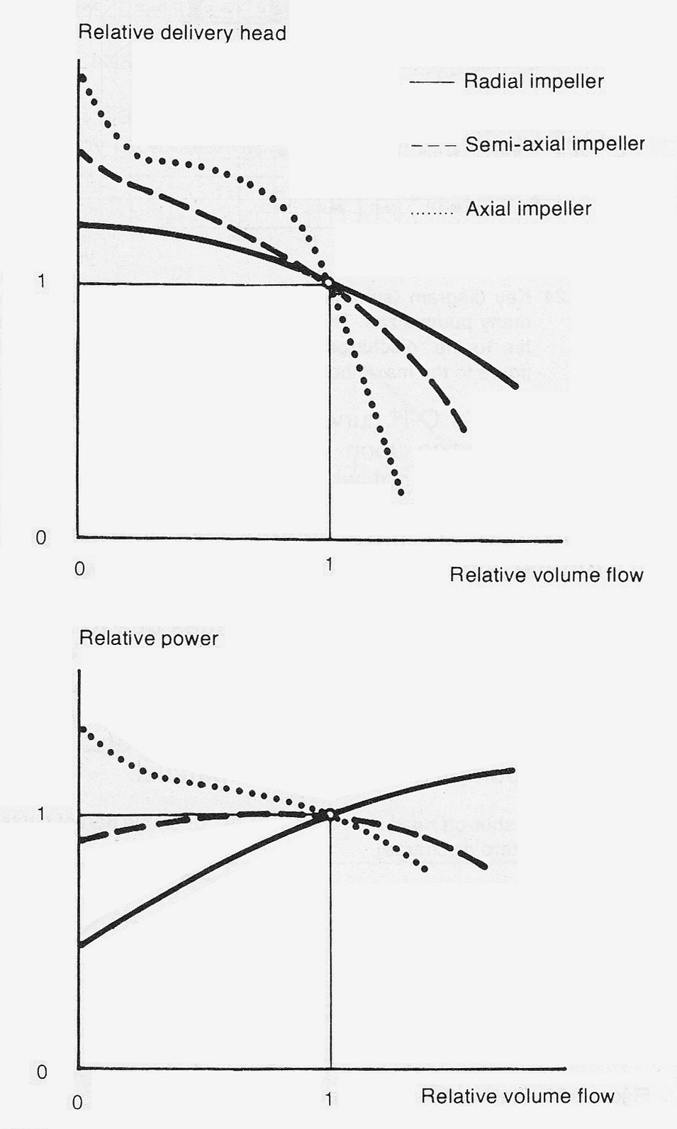
Figure 3.16d Centrifugal pump curves expressed relative to the maximum efficiency point for different types of rotor dynamic pumps.
The shape of the power curve is, together with variations in the volume flow transported, the determining factor for size of the drive motor. In the case of axial pumps, see figure 3.16d, the greatest power requirement is when the flow is zero, which can mean that the pump starting relationship must be adapted to this fact. In the case of centrifugal pumps the power requirements which are given in the pump catalogues, unless otherwise stated, refer to liquids comparable with cold water, i.e. with a density of 1000 kg/m³.
In the case of liquids having different densities from that of water, the use of the unit, “m” can cause misunderstanding.
The unit “m” stands for meter liquid column. If reference is made to meter water column it is suitably written mH20 so as to avoid confusion. The reason for this confusion is that a centrifugal pump give the same delivery
head in meter liquid column (m), irrespective of the density of the liquid. The pump power requirement is on the other hand proportional to the density. For densities different from that of water the power requirements quoted in the purchasing documents always relate to the liquid stated. In cases of doubt, double power requirements should be stated whereby that for water is only valid during acceptance testing. The code for acceptance testing of turbine pump performances as compared to the manufacturer guarantee is covered by current (ISO) standards. The guarantees in this case relate to a normal set-up. An unsuitable design of, above all, the inlet pipe in an installation can alter performance.
A centrifugal pump performance falls off with wear of the actual pump parts. This wear occurs both at the positive element clearances, affecting the internal leakage (slip), figure 3.1b>>>, and at the blades, decreasing the blade work, figure 3.16f. It is very difficult to give a limit for the extent of wear but reductions in delivery head of the order of 10% during the pumping of pure liquids are, however, considered to be tolerable.
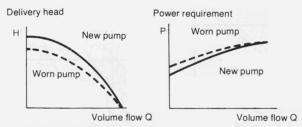
Figure 3.16e The effect on performance of wear in sealing clearances.

Figure 3.16f Effect of wear on pump blades.
The performance of centrifugal pumps falls rapidly with increasing viscosity of the pumped liquid. This reduction expresses itself in such a manner that the Q-H curve falls but shut-off head is retained. The power requirement rises considerably primarily due to the increase of impeller friction. Figure 3.16g shows examples of the alteration of performance for smaller centrifugal pumps. In the case of larger centrifugal pumps, this effect of viscosity is not considerable until viscosity has risen by a factor of 10.

Figure 3.16g Examples of the effect of viscosity on a smaller radial pump, nq = 11 r/min., discharge dimension 50 mm. Max efficiency (not shown) falls from approx 50% to approx 5%.