9.2 Branched pipe system
Branched pipe system
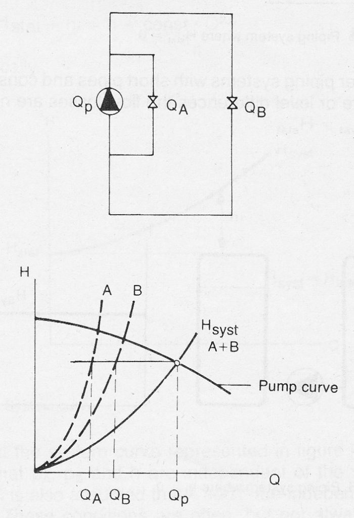
The first example of a branched pipe system is a circulation system. In such a case Hstat = 0. The volume flow QP, which passes through the pump, is divided at the branch point. Continuity dictates that
QP = QA + QB (Equ. 9.2a)
Both branches A and B have their own system curves, the sum of which determines the resultant system curve. The intersection point of the resultant system curve and the pump curve determines the pump’s optimum operating point.

Figure 9.2a Branched circulation system.
Figure 9.2a also shows how large a portion of the pump flow flows through each respective branch. The division of flow depending upon the magnitude of the losses in each respective branch. In this example it is assumed that the branch point is near to the pump i.e. that flow losses between the pump and the branch point can be neglected.
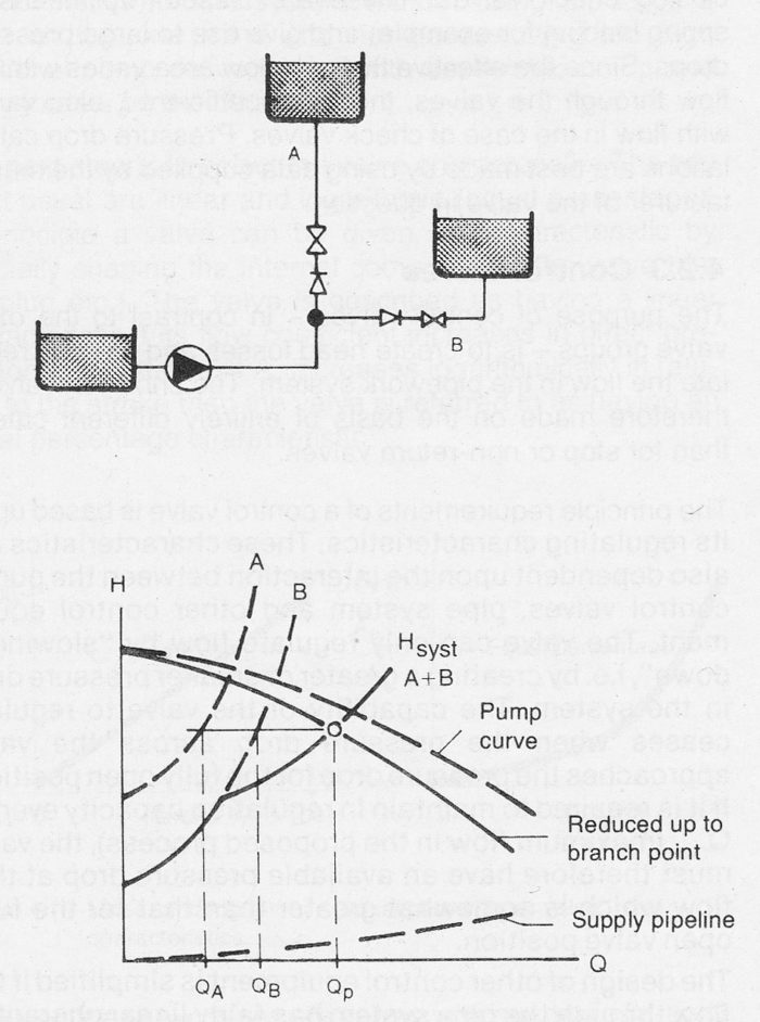
Figure 9.2b Branched pipe system, Hstat = 0
The next example, figure 9.2b, also takes into consideration the losses in the main pipeline up to the branch point. This is done by reducing the pump curve by the magnitude of the losses up to the branch point. The “reduced” curve is then matched to the remaining system curve as before.
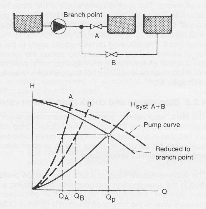
In the third example the pump curve is first reduced to the branch point. Thereafter the system curves A+B are added to the resultant system curve Hsyst A+B. The intersection point between the reduced pump curve and the resultant system curve determines the pump operational point, as shown in figure 9.2c.

Figure 9.2c Branched pipe system with static delivery head.
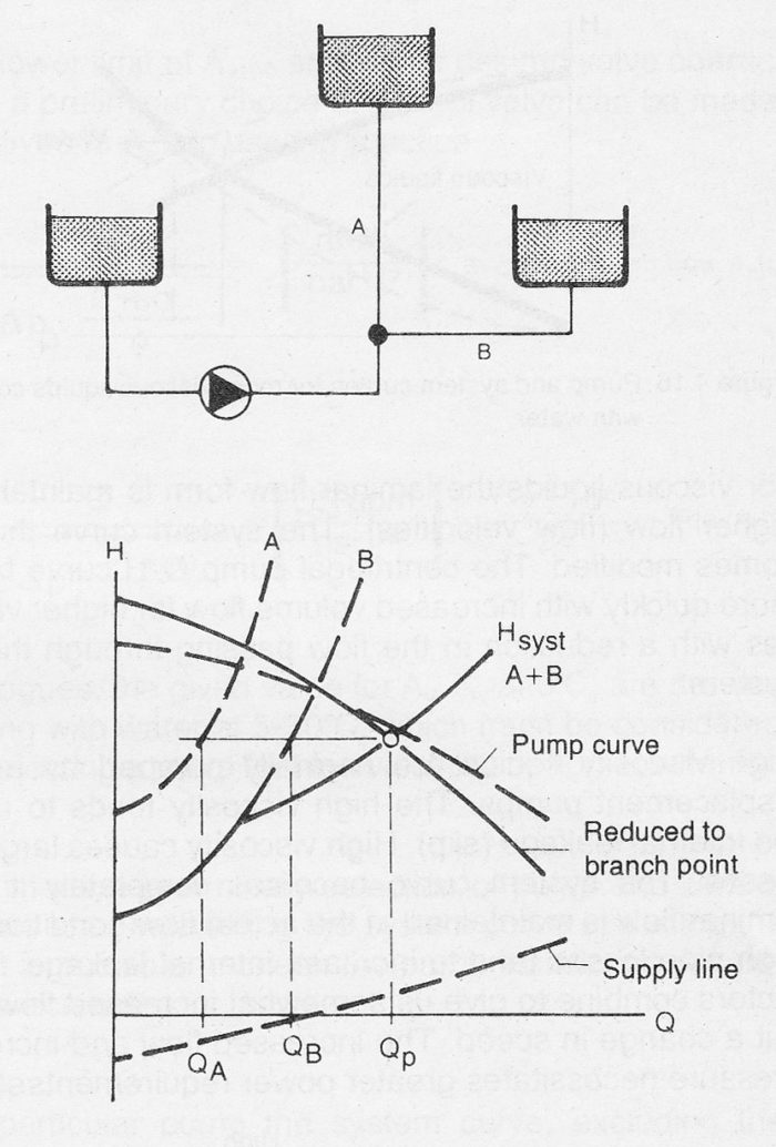
In the fourth example there is a level difference (in this example a supply head) between the supply vessel on the suction side and the branch point. The system curve for the supply pipeline exhibits therefore, a static head (Hstat < 0).
The method is the same as in the previous examples. First reduce the pump curve with the supply line curve up to the branch point. Then determine the system curves for the branches A+B from the branch point. The resultant branch curve is then matched to the pump’s reduced curve as shown in figure 9.2d.

Figure 9.2d Branched pipe system with falling supply line.
This method can be applied in principle to calculate any pipework system, however complicated and containing any number of branch points. The first step is to determine the resultant system curve for the branch furthest from the pump in relation to the furthest branch point. The next step is to deal with the next branch point and so on until the branch point nearest to the pump is reached.
A common problem is to dimension a piping network with many branches and many tapping points in such a way as to guarantee a predetermined capacity at each tapping point. Dimensioning is carried out so that the pipeline requiring the most pressure, usually the pipeline to the furthest tapping point, is dimensioned first. The branch lines are then calculated on the basis of the excess pressure available at the branch points. The excess pressure at the branch points can be such that it is necessary to equip a branch line with extra throttling to prevent it from “stealing” capacity from the other tapping points.

