
8.12 Pressure loss nomogram and diagram
Pressure loss nomogram and diagram
Pre computed pressure loss nomogram and diagram in pipes for a number of commonly applied cases of flow are set out in this section in the form of diagrams. These diagrams and nomograms can be used to calculate the losses in a system, i.e. flow losses in the pipes, valves, bends, etc. This method is quick and provides acceptable results if carried out accurately. A number of diagrams for the determination of the associated values of velocity, frictional losses, diameter and volume flow are presented. There are also diagrams for determining the flow velocity in cylindrical conduits in relation to the volume flow and diameter together with diagrams for the determination of loss of head (m) in bends fittings etc., related to the velocity of flow.
It is most practical when dimensioning pipes to be able, right from the outset, to assess the approximate economic flow velocity. By this means, the final economic dimensioning can be carried out more quickly, since fewer alternatives then have to be tested. Figure 8.12a gives guideline for normal flow velocities in some common cases.
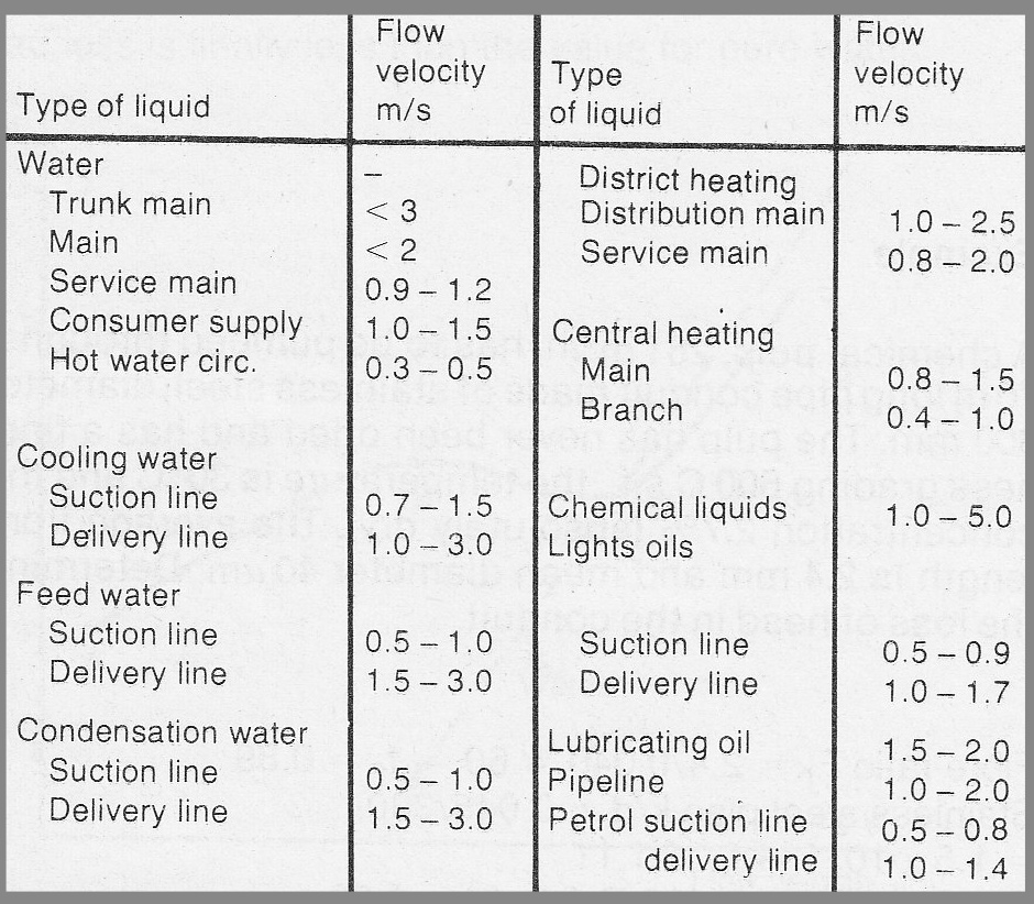
Figure 8.12a Guideline flow velocities for general applications.
High flow velocities give small pipe dimensions = low plant procurement costs, but cause greater pump power consumption through greater frictional losses = high running costs.
Quite apart from economy, other factors can effect the choice of flow velocity; noise in central heating equipment, erosion in copper hot water pipes; static electricity for liquids with low flash points; risk of cavitation in suction lines at high temperature and with sudden changes in velocity; sedimentation with solid suspensions, i.e. critical velocity.
Losses in bends, valves etc. can be expressed as equivalent straight pipe lengths by using the values in figure 10.12b. The values for valves are mean values and vary according to the design.
By adding the equivalent length of pipe and the “real’ length, the total pipe length is obtained enabling the flow losses, expressed as head (m), to be calculated from the diagrams.

Figure 8.12b Conversion factors for equivalent pipe lengths, (guideline values)
As pointed out in Section 8.6 >>> , the equivalent pipe length depends upon the straight pipe loss coefficient λ, i.e. pipe roughness, Reynolds number etc. The numerical values in figure 8.12b, therefore, must be regarded as approximate guideline values.
Alternatively, losses in bends, valves etc.. can be separately calculated by converting the values for ζ (zeta) obtained from figure 8.6c into metres head (column of liquid) at specific flow velocities with the help of the diagrams.
Note that the stated value of ζ is for turbulent flow. In the case of laminar flow, conversion to equivalent pipe length is the handiest way to calculate these losses.

Figure 8.12c Index of diagrams for calculating pressure losses in pipelines.
The applicability of the diagrams is greater than the impression given by figure 8.12c. The diagrams for water can be used for all water-like Newtonian liquids, i.e. for liquids with corresponding viscosity. Note, however, that if the pressure loss is stated in Pa (Pascals) the density must also coincide with that of water.
The diagrams for oils can be used for all Newtonian liquids with higher viscosities than water, under the same conditions.