
9 Pump system
Pump system
This section about pump system deals with the interaction of pumps and other components in a piping system. The chapter is primarily directed to the sizing parameters while operational parameters are dealt with in Chapter 10.
In order to determine the required pump performance it is first necessary to define the characteristics of a particular pipework system (installation). This applies to single pipe systems as well as branched systems. An appreciable portion of the pressure losses in the system are caused by valves, especially control valves in throttle-regulated installations. Pumps working in a system operate in conjunction with the pipework and other components to deliver the required flow. Final choice of pump size must be made with due regard to the pump efficiency curve and the hydraulic tolerances of the installation components. The chapter finishes with an explanation of the water hammer (pressure surge) phenomenon. Easily calculated estimations are given to show when the risks of water hammer are present and when the use of protective equipment is necessary. Various types of protection devices are reviewed.
System curves and pump nominal duty point or operating point
When connected in a pipe system a pump will operate at a point of equilibrium between the pump and the pipe system. At the point of equilibrium the driving function of the pump is equal in magnitude to the resistance in the system. The pump characteristics in this respect are usually represented by the Q-H curve. The equivalent curve for the pipe system is called the system curve and is designated Hsyst.

Figure 9a Pump optimum operating point
The volume flow at which the pump and system curves intersect each other, is the flow which will pass through the pipe system. In order to correctly determine the size and dimensions of the pump and pipe system a knowledge of the characteristics of their respective curves is necessary. This section deals With the characteristics of the pipework system.
Figure 9a shows typical curves for a centrifugal pump with a low specific speed (radial pump) when pumping a water like liquid. The curves vary in shape when pumping other liquids and when using other types of pumps. Generally, however, the flow is always determined by the balance between the pump and system.
Single pipe system
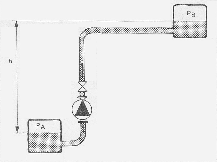
Figure 9b Example of single pipe system
The system delivery head is usually divided into a static component Hstat and a loss component hL.
Hsyst = Hstat + hL (Equ. 9a)
The static component, which is assumed to be independent of volume flow, comprises of the difference in static pressures and the level differences between the boundaries of the system. Using the designation as in figure 9b:

P = static pressure (N/m²)
ρ = density of liquid (kg/m³)
g = acceleration of gravity 9,086 (m/s²)
h = level difference (m)
The losses include flow losses in straight pipe and losses in valves and fittings etc.
hL = h(straight pipe) + h (fittings and valves) (Equ.9c)
Using the terms as defined in Chapter 8.8 >>>
Total head loss in pipe system consist of the sum of the straight pipe head losses and the head losses in fittings, valves and other components.
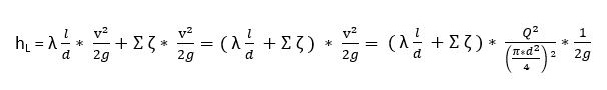
hL = head loss (m)
λ = loss coefficient for straight pipe (also known as Darcys friction factor)
ζ = loss coefficient for fittings, valves etc.
Σζ = sum of all loss coefficients
l = length of pipe (m)
d = diameter of pipe (m)
Q = volume flow (m³/s)
v = flow velocity (m/s)
For a given pipework system (l, d) With water-like liquids the loss coefficients λ and ζ are often (large Re) independent of Q. The loss of head then becomes:
hL = constant * Q²
The pressures at the system boundaries are such that PA = PB = atmospheric pressure. So that Hstat equals the level difference (h), the system delivery head then becomes:
Hsyst = Hstat + hL = h + constant * Q²
or graphically
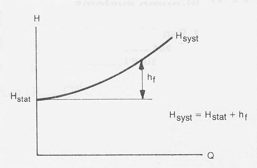
Note that the system curve represented in figure 9c assumes that PA, PB and h are independent of the volume flow Q. lt is also assumed that λ and ζ are independent of Q (Re). These conditions are often, but not always, fulfilled.